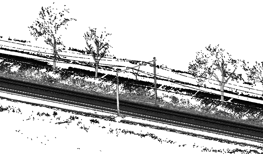
Modern Mobile Mapping systems make it very easy to quickly map large areas. Current laser scanners with pulse rates of 1 MHz and above make it possible to achieve sufficient point density even at highway driving speeds. Under good GNSS circumstances, post-processed trajectory accuracies of a few centimeters can be achieved without the need for ground control points. But a single driveline is usually not sufficient for full data coverage, be it due to occlusion from other vehicles or the need to zig-zag through all roads of a residential area.
If a homogeneous point cloud is required, as is often the case, this requires relative adjustment of overlapping drivelines onto each other. This is not a trivial task, despite the claims of some hardware and software vendors. This article tries to explain some of the challenges involved and how I tackle them in my own software. It is based upon my experience with processing Mobile Mapping data in both road and rail environments, with Riegl and Leica Mobile Mapping systems and their respective processing packages.
Finding suitable geometry
Relative adjustment requires geometry that is present in all overlapping drivelines and that is suitable for matching in both height and X/Y. A common approach is to detect planar geometry, which is easily achieved by eigenvector/eigenvalue analysis of point neighbourhoods. Adjustment is then possible in the direction of the normal vector of the plane.
A problem arises when there is insufficient planar geometry available. Height adjustment is generally not an issue but, depending on the desired size of the planes, it can be difficult to find vertical planes that are suitable for X/Y matching outside of built-up areas. This is especially the case with rail applications, where very high matching quality is required.The advantage of the planar approach is that it also allows for improvement of the orientation angles, which is especially useful with dual-scanner systems.
Another approach is to extract cross sections and match these in 2D, which in theory is a relatively simple operation that can be implemented with image processing algorithms. But this also requires sufficient vertical features in a cross section, and I’ve seen an implementation that completely failed to even match height when there was no vertical geometry available, limiting its suitability to urban areas.
Another issue is geometry that is scanned from different sides. Below image shows a top view a wall with a fence on top scanned from two sides. If these two point clouds were blindly matched upon each other, a very thin wall would result…

Proper weighting for maximum accuracy
Matching point clouds should never be a case of simply averaging all differences or randomly selecting one driveline as reference and forcing the others onto it. Luckily, it is common practise to apply relative weighting based upon the position accuracy as reported by the trajectory processing software. Issues arise when these accuracies are not correct. They are simply the estimated accuracies as reported by the Kalman filter and depend upon the stochastic model and the GNSS situation, but do not take into account errors like multi-path and cycle slips. That’s why I prefer the separation (the difference between forward and backward computation of the Kalman filter) as accuracy measurement above the estimated position accuracy.
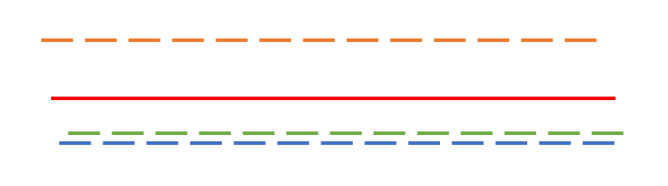
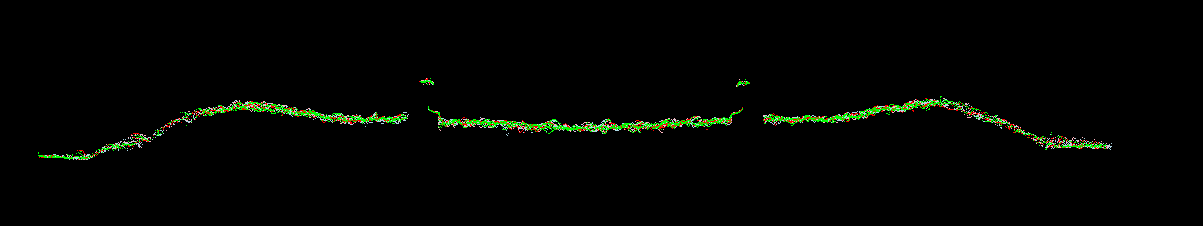
Below figure shows what happens in the case of three drivelines (dashed) with similar reported accuracies, but one of having a systematic offset due to an outlier, which could e.g. be a bad ambiguity fix. The resulting averaged trajectory (solid) is not where it should probably be, namely closer to the two other drivelines.
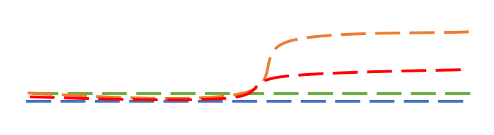
Such situations can be rectified by a sufficiently dense network of ground control points. But matching with improper weights can also destroy your relative accuracy. In the figure below, one driveline suddenly deviates from the others, causing a large deformation of the adjusted trajectory over a short distance. This could only be rectified by ground control points immediately before and after the occurrence of the deviation.
Avoiding error propagation
Ideally drivelines overlap over their entire length , which makes it possible to adjust them along their length at small intervals. This is however difficult to achieve in urban areas where drivelines only overlap at intersections. If corrections are interpolated linearly between overlapping locations, errors/differences present at one location may get propagated over a larger area.
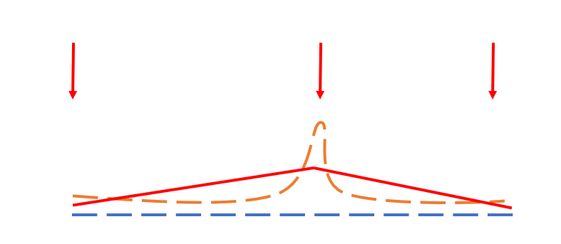
Below figure show a situation with three matching locations (the arrows), with one driveline having a large error in a limited area which happens to coincide with the middle matching location. If the differences/corrections are interpolated linearly, they will be propagated to a much larger area than necessary. This is a scenario that I’ve encountered several times, and this might be the reason why Riegl’s RiPrecision limits the effect of a correction to 10 seconds.
The HaiQuality Adjust approach
The issues mentioned above have made me write my own software for matching of Mobile Mapping point clouds, which in its current incarnation is called HaiQuality Adjust. It is not perfect and requires manual intervention, but it provides full control over the entire process. The key features are described here:
Full transparency
I have a major dislike of black box algorithms and software vendors saying that what their software does is “secret”, but that I can trust them that it is doing what it is supposed to do. HaiQuality Adjust provides full control over all steps of the matching:
- Definition of adjustment locations. This can be done manually, or automatically along a given axis or by first finding suitable geometry in the point clouds. These steps are done in QGIS, so it is easy to e.g. draw the locations upon aerial imagery.
- Selection of point clouds/drivelines to be matched. This is also done in QGIS, enabling to user to easily deselect drivelines that are not of interest.
- Cutting of point clouds. The parts of the point clouds that are to be used for matching are cut from the point clouds, which means that they don’t have to be traversed during computations or visual control.
- Matching. This is done using a point-to-plane ICP (iterative closest point) algorithm that runs on the GPU.
- Visual control. Each location can quickly be controlled visually and matches corrected manually if necessary.
- Analysis of corrections. Computed corrections are tested against the estimated accuracies, making it possible to identify drivelines of lower accuracy and downweight them or deselect them altogether.
- Application of corrections. This is done with an external program that directly applies corrections to the points, interpolating linearly based upon timestamps.
2D and 3D
The default matching mode is 3D, using a point-to-plane ICP algorithm for matching overlapping point clouds onto each other. This works very well in the presence of sufficient planar geometry. Especially for rail applications, this might not be sufficient to achieve a very high relative accuracy, where matching at smaller intervals (e.g. every 10m) might be desirable. For this purpose, a 2D mode is also implemented that extracts and matches cross sections.
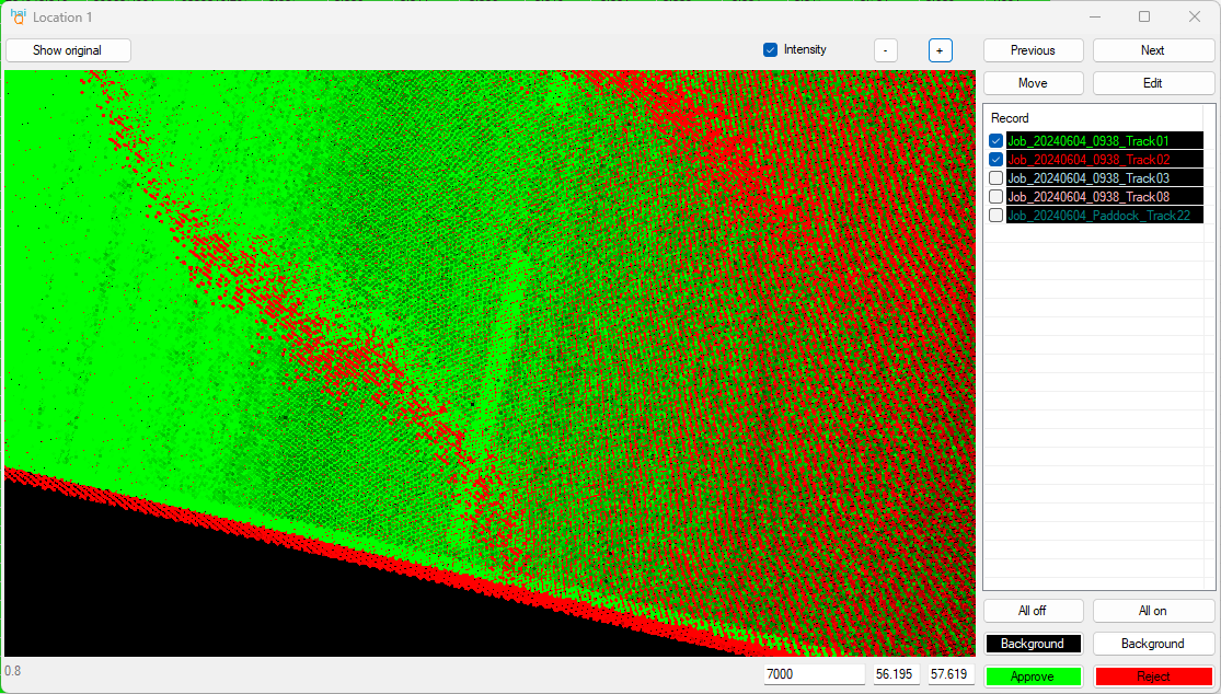
Fast visual control
Due to the issues described above, automatic processing will never be 100% perfect. That’s why I consider manual checking and improvement of matching results an essential ingredient of a workflow for projects with high accuracy requirements. HaiQuality Adjust makes it possible to do this efficiently via key shortcuts to quickly view a point cloud from all sides and move drivelines onto each other. Corrections are directly recomputed, meaning that what you see is what you get. Intensity-based display even makes it possible to manually match road point clouds by paint lines in the absence of vertical geometry. It is also possible to identify locations that deviate from their neighbours, meaning that you don’t need to check everything but only the outliers, which is especially important for the 2D mode.
Testing of stochastic model
Even perfect matching yields suboptimal absolute and relative accuracy if the stochastic model used for the relative weighting is incorrect. The estimated position accuracies are often too optimistic. To deal with this, HaiQuality Adjust computes the normalized residual, i.e. the correction divided by the standard deviation, as testing criterion. Large normalized residuals are indicators of a stochastic model that is too optimistic. Affected drivelines can be downweighted by increasing their standard deviation, or deselected altogether. Even if deselected, they will still be adjusted, but they no longer take part in the computation of the corrections and thus have no negative impact on the accuracy.
No reprocessing required
Some software packages require you to reprocess and export all data after matching. This is not the case with HaiQuality Adjust. The result is a text file consisting of time stamps and corrections in X, Y, and Z direction. These corrections can be directly applied to point clouds and external orientation files for images. If desired, it is also possible to generate a new trajectory file.
Suitable for relative and absolute adjustment
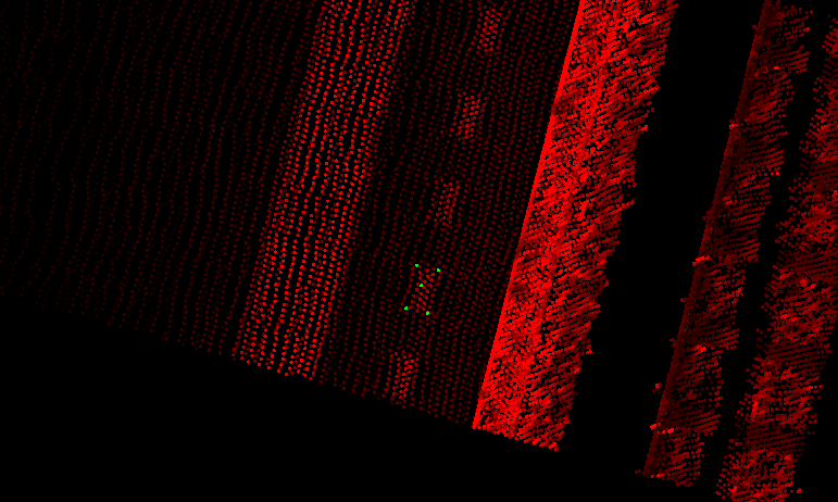
While this article has focused on relative matching, HaiQuality Adjust is also suitable for absolute matching onto ground control points, which can be either point-wise measurements (like those obtained with GNSS or total stations) of laser scans. Adjustment onto laser scans can be done with the above-mentioned ICP algorithm, whereas matching onto points requires manual intervention. Below screenshot shows the use of the corners of white tiles on a platform as GCPs.
Vendor independent
HaiQuality Adjust is vendor independent. All it requires are a trajectory file with timestamps, positions, and accuracies, and the point clouds in LAZ format. Currently implemented are the direct use of trajectories in Riegl and Inertial Explorer format, and other formats can easily be implemented.
Limitations
No software is perfect, and this also holds for HaiQuality Adjust. Here are the most important limitations:
- Manual checks are required, as the matching is not always perfect in the absence of suitable geometry or insufficient overlap between drivelines. Due to this it is more suitable to projects with high accuracy requirements than large-scale processing.
- Currently no corrections to the orientation are estimated.


2 gedachten over “Why relative adjustment of Mobile Mapping data is difficult”